

Interactive visualization tool for (meta)genome assembly graphs.
MetagenomeScope decomposes the graph into structural patterns and highlights these as annotations on the graph. By default it lays out the graph hierarchically, using Graphviz' dot algorithm. These and other approaches help simplify the investigation of fine-grained structures within assembly graphs.
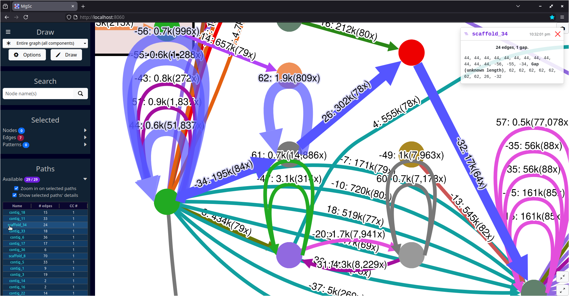
MetagenomeScope also contains various functionalities for visualizing assembly graphs at larger scales -- for example, highlighting scaffold paths on the graph and drawing summary plots of the graph's structure.
MetagenomeScope supports the outputs of most modern assemblers, can handle large graphs including tens of thousands of nodes, and is backed by over five hundred automatic software tests.
The tool is under active development, so please let us know if you have any feedback!
| Stool metagenome assembly (MetaCarvel) |
 |
| Data source: SRS049959 |
| Human genome assembly (HG002, Verkko v1.1) | Yeast genome assembly (Flye) |
|---|---|
 |
 |
| Data source: T2T Consortium | Data source: AGB |
| Summarizing graph structure in a treemap | Interactive charts of graph statistics |
|---|---|
 |
 |
| Data source: SRS049959 | |
mamba install -c bioconda -c conda-forge metagenomescopeUsing pip
First, you need to make sure that Graphviz
and PyGraphviz are installed
properly (so that PyGraphviz knows where to find Graphviz).
See PyGraphviz'
INSTALL.txt
for details.
(Probably the most consistent way to do this is just installing Graphviz and PyGraphviz from conda-forge, but at that point you might as well do the entire installation from within conda...)
Anyway, once Graphviz and PyGraphviz are installed, you should be able to just run:
pip install metagenomescopemgsc -g graph.gfa... where graph.gfa is a path to the assembly graph you want to visualize
(see information below on supported graph filetypes).
This will start a server using Dash.
The port number of the server defaults to 8050, so navigate
to localhost:8050 in a web browser to access the visualization.
Usage: mgsc [OPTIONS]

  Visualizes an assembly graph.

  Please visit https://github.com/marbl/MetagenomeScope for more information.

Options:
  -g, --graph FILE          In GFA, FASTG, DOT, GML, or LastGraph format.  [required]
  -a, --agp FILE            AGP file describing paths.
  -t, --vtsv FILE           Verkko assembly.paths.tsv file describing paths.
  -i, --info FILE           Flye assembly_info.txt file describing contigs/scaffolds.
  -p, --port INTEGER RANGE  Server port number.  [default: 8050; 1024<=x<=65535]
  --rmdup [gfaonly|y|n]     Remove parallel edges.  [default: gfaonly]
  --decomp / --no-decomp    Do pattern decomposition.  [default: decomp]
  --dcheck / --no-dcheck    Do post-decomposition sanity check.  [default: no-dcheck]
  --debug / --no-debug      Use Dash's debug mode.  [default: no-debug]
  --verbose / --no-verbose  Log extra details.  [default: no-verbose]
  -v, --version             Show the version and exit.
  -h, --help                Show this message and exit.
| Filetype | Generated by | Notes |
|---|---|---|
GFA (.gfa) |
Flye, LJA, hifiasm, Verkko, ... | Both GFA 1 and GFA 2 files are accepted. Currently we visualize segments (S-lines), links (L-lines in GFA 1), dovetail edges (some E-lines in GFA 2), and paths of segments (P-lines in GFA 1, O-lines in GFA 2). |
FASTG (.fastg) |
SPAdes, MEGAHIT | Expects FASTG files produced by SPAdes or MEGAHIT. |
DOT (.dot, .gv) |
Flye, LJA | Expects DOT files produced by Flye or LJA. See "What filetype should I use for de Bruijn graphs?" in the FAQs below. |
GML (.gml) |
MetaCarvel | Expects GML files produced by MetaCarvel. |
LastGraph (.LastGraph) |
Velvet | Currently we just visualize the raw structure (nodes and arcs). |
Should you run into additional assembly graph filetypes you'd like us to support, feel free to open a GitHub issue.
Paths can optionally be specified through any of the following inputs:
AGP files (-a)
See the AGP specification for details.
If your graph is in DOT format:
- We assume the
component_ids in column 6a of the AGP file correspond to edge IDs.
Otherwise:
- We assume the
component_ids correspond to node IDs.
Verkko assembly.paths.tsv files (-t)
See Verkko's documentation for details.
If your graph is in DOT format:
- We assume names on each path correspond to edge IDs.
Otherwise:
- We assume names on each path correspond to node IDs.
Flye assembly_info.txt files (-i)
See Flye's documentation for details.
If your graph is in DOT format:
- We will visualize the edge-paths described in the
.txtfile.
If your graph is in GFA format:
- If there are node names in the GFA file that match up with row names in the
.txtfile, we will extract information from the.txtfile (e.g. coverage) and show it in the interface as node data.
If your graph is not in DOT or GFA format:
- We will ignore the
.txtfile. (Since Flye should only generate DOT or GFA assembly graphs, at least to my knowledge?)
P-lines in GFA 1 files, or O-lines in GFA 2 files (-g)
For GFA 1 paths (P-lines):
- We will visualize these node-paths.
For GFA 2 paths (O-lines):
-
We will show all of the nodes on these paths, "expanding" edges and recursive patterns accordingly.
-
For more details, see "How do you handle
O-lines in GFA 2 files?" in the FAQs below.
MetagenomeScope hierarchically detects and highlights five types of structural patterns on the graph:
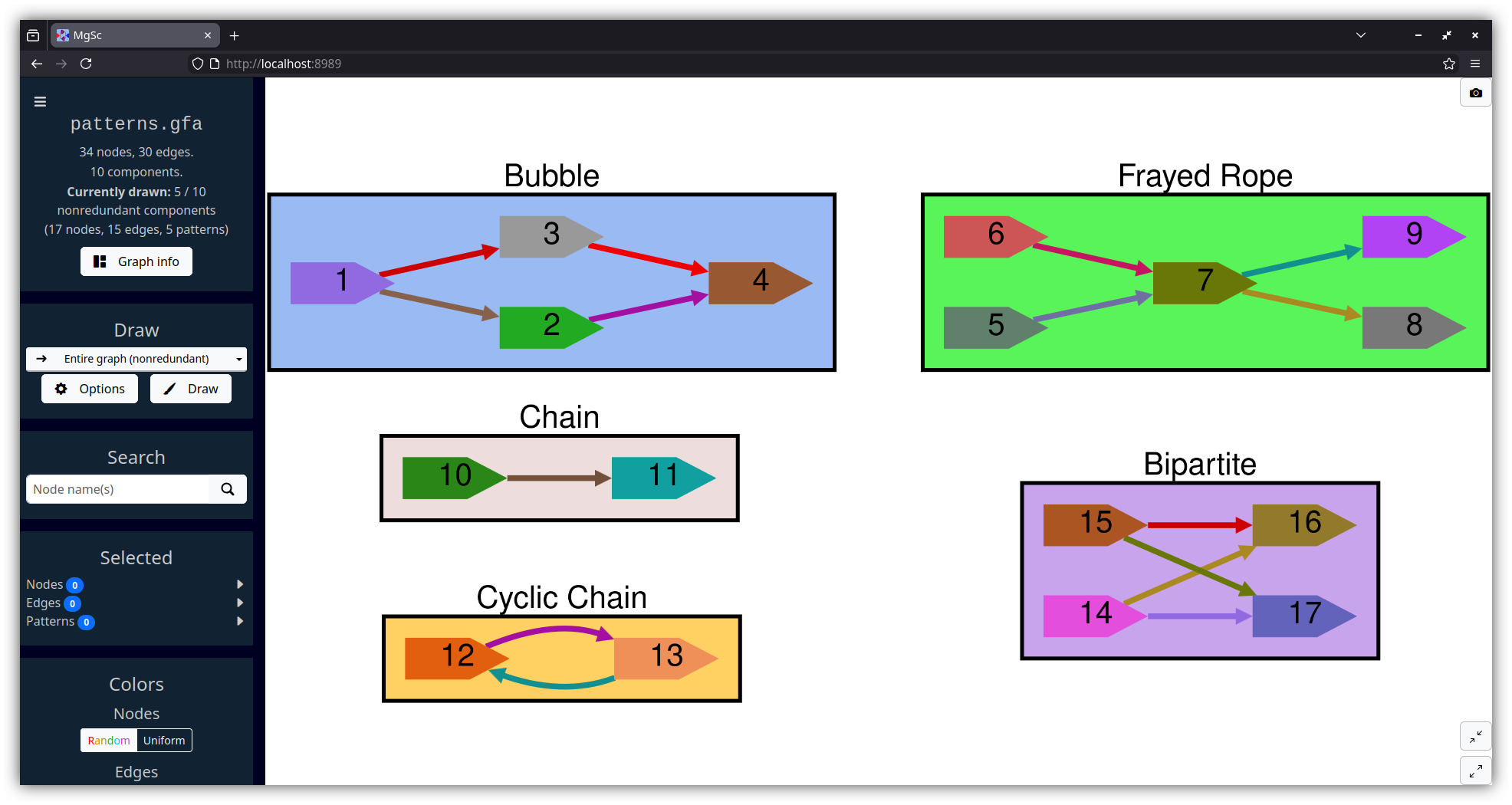
Bubbles (Miller et al., 2010; Nijkamp et al., 2013) follow a diverge-coverge pattern. They generally indicate variation -- either real (e.g. an alternate path is caused by a SNP) or erroneous (e.g. an alternate path is caused by a sequencing error). We identify bubbles using a modified version of the algorithm given in Onodera et al., 2013.
Similarly, bulges (Pevzner et al., 2004; Vasilinetc et al., 2015) are pairs of nodes where there exist multiple parallel edges from one node to another.
Bulges can typically be interpreted the same way as bubbles -- you generally see bulges in "edge-centric" (e.g. de Bruijn) graphs, and bubbles in "node-centric" (e.g. overlap) graphs. So, we label both bubbles and bulges identically.
Frayed ropes (Miller et al., 2010) follow a converge-diverge pattern; they have the opposite structure as bubbles. They generally indicate interspersed repeats in the middle region.
Chains are just non-branching paths of at least two nodes. Cyclic chains are chains where the end node has an outgoing edge to the start node. Cyclic chains represent a simpler form of what are known in edge-centric graphs as whirl structures (Pevzner et al., 2004).
Bipartites are regions of the graph that can be partitioned into two layers of nodes (let's call them Left and Right), such that all of the nodes in Left have outgoing edges to all of the nodes in Right. We require that both Left and Right contain at least two nodes each. (Such a pattern is essentially a stricter version of a complete bipartite graph.)
Surprisingly, bipartites pop up a lot in certain assembly graphs! These are less well-documented in the literature than the above types of patterns, but our suspicion is that these are another indication (like frayed ropes) of repeats -- and that a lot of these patterns in succession might indicate things like strain heterogeneity. See Figure 5 of Li et al., 2012 for an example of how a bipartite (or, viewed another way, a frayed rope) could be caused by a repeat.
Sometimes, it is best to consider a node as the child of two patterns. A common example of this is a bubble chain (Dabbaghie et al., 2022), where multiple bubbles occur one after another. In a bubble chain, the "end node" of one bubble is also the "start node" of another bubble!
To accommodate these kinds of cases, MetagenomeScope splits the boundary nodes of a pattern.
Splitting a node A transforms it into two nodes: A-L and A-R, which are connected by a single "fake edge" A-L -> A-R.
Because this allows a node to be in two patterns simultaneously, this makes it possible for us to identify a much richer set of patterns and describe the graph structure more accurately.
"Split nodes" and "fake edges" are drawn with distinct visual styles, in order to make them clearer -- split nodes are drawn in a way that looks like the node has been split in half, and fake edges are drawn as thick dashed lines.
| Split nodes in a node-centric graph MetaCarvel stool metagenome scaffold graph (the "large graph" shown below), component #17 |
 |
| Split nodes in an edge-centric graph jumboDBG de Bruijn graph of human chromosome 15 (available as chr15_full.gv in metagenome/tests/input/) |
 |
Note that node splitting is not always necessary -- as the figures above show, sometimes a boundary node of a pattern doesn't need to be the boundary node of any other pattern. To limit the amount of split nodes we need to show in the visualization, we detect and remove unnecessary split nodes after finishing the decomposition procedure.
Here are three graphs of various sizes, each produced by a different assembly program.
This data is from AGB's GitHub repository.
wget https://raw.githubusercontent.com/marbl/MetagenomeScope/refs/heads/main/metagenomescope/tests/input/flye_yeast.gv
wget https://raw.githubusercontent.com/marbl/MetagenomeScope/refs/heads/main/metagenomescope/tests/input/flye_yeast_assembly_info.txt

mgsc -g flye_yeast.gv -i flye_yeast_assembly_info.txt| Entire graph |
 |
| Zoomed in on scaffold_34 in component #1 |
|
Tip
The "Labels" section of the interface has some settings that help make labels prettier. I produced the screenshot on the right above using the Offset, Outline, and Rotate edge label settings.
Note
We draw DOT files from Flye and LJA using the typical conventions for drawing de Bruijn graphs -- with nodes represented as circles, and edges given labels with their length and coverage. This resembles the styles from various papers that show visualizations of these kinds of graphs, including Pevzner et al., 2004; Mikheenko & Kolmogorov 2019; and the DOT outputs of Flye and LJA.
This is an example graph from Bandage.
wget https://github.com/rrwick/Bandage/raw/refs/heads/gh-pages/samples/E_coli_LastGraph.zip
unzip E_coli_LastGraph.zip

mgsc -g E_coli_LastGraph| Hierarchical layout with dot |
 |
| Force-directed layout with sfdp (not showing patterns, and using an overlap scaling factor of -15) |
 |
Note
As discussed in the FAQs below on "Reverse-complementary sequences," we represent pairs of nodes {X, -X} and pairs of edges {A -> B, -B -> -A} separately in the graph. This makes it easier to lay out the graph nicely.
In graphs where such pairs of nodes / edges exist, there will be an additional drawing option available (under the "Draw"
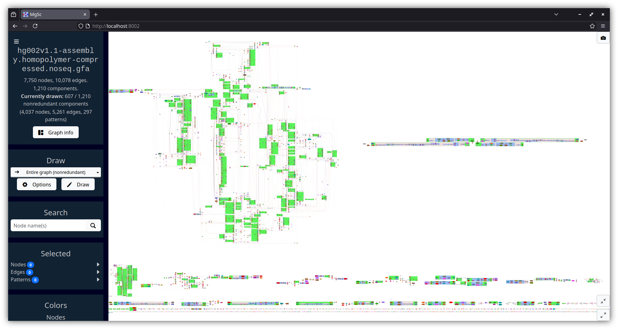
section of the UI) named Entire graph (nonredundant).
This drawing option will detect "redundant" pairs of connected components that are perfectly
reverse-complementary to each other (e.g. one component looks like A -> -B -> C and the other looks like
-C -> B -> -A), and only draw one of these components (we select the component with more forward-orientation nodes or edges).
This drawing option will also draw components that have no perfect reverse-complement component -- for example, those that are "strand-mixed"
and contain both node X and -X (e.g. component #1 in the above screenshots).
You can think of this drawing method as kind of a mix of the "single" and "double" modes in Bandage. For pairs of redundant components, we only need to draw one of them, and for all other components we draw the entire thing.
If you want to see everything, just select the Entire graph (all components) drawing option!
This is a scaffold graph created by MetaCarvel.
Here is a Zenodo record for these files;
they are derived from SRS049959.
Note that this graph is fairly old (it dates back to August 2017!); MetaCarvel has been updated a decent amount since then.
wget https://zenodo.org/records/18316065/files/august1.gml
wget https://zenodo.org/records/18316065/files/scaffolds_august1_fixed.agp

# Use --verbose to show more information in the terminal about how long each step takes
mgsc -g august1.gml -a scaffolds_august1_fixed.agp --verbose| Entire graph (on my 2018 laptop this takes about 2.5 minutes to lay out and draw; see tip below) |
 |
| Zoomed in on scaffold_1486 in component #65 |
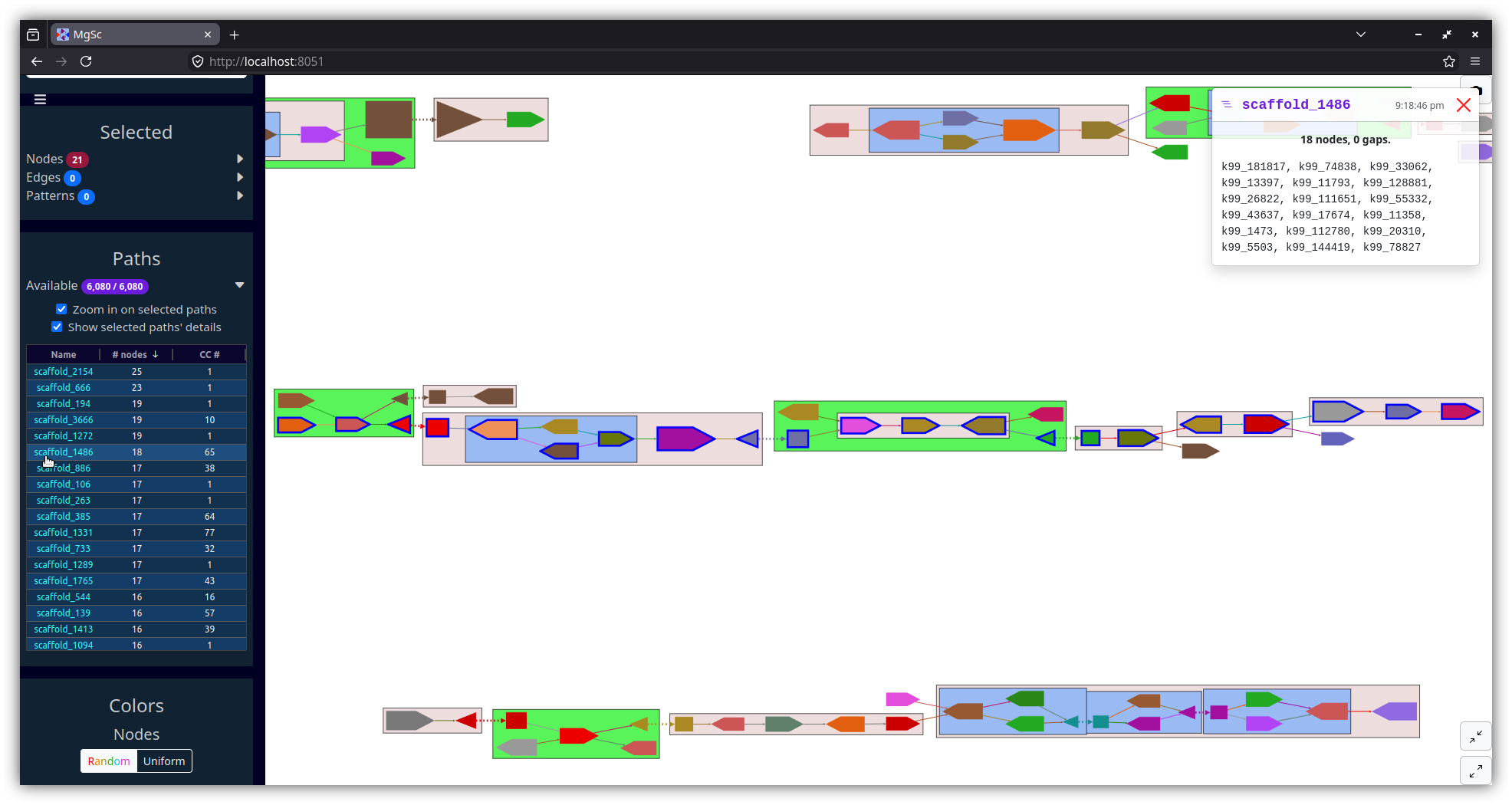 |
Tip
If you are working with a big graph like this, immediately pressing the "Draw" button (to lay out and draw the largest connected component, #1) may not be a good idea. Some steps you can take to get a sense of the graph structure without having to immediately draw a bunch of things:
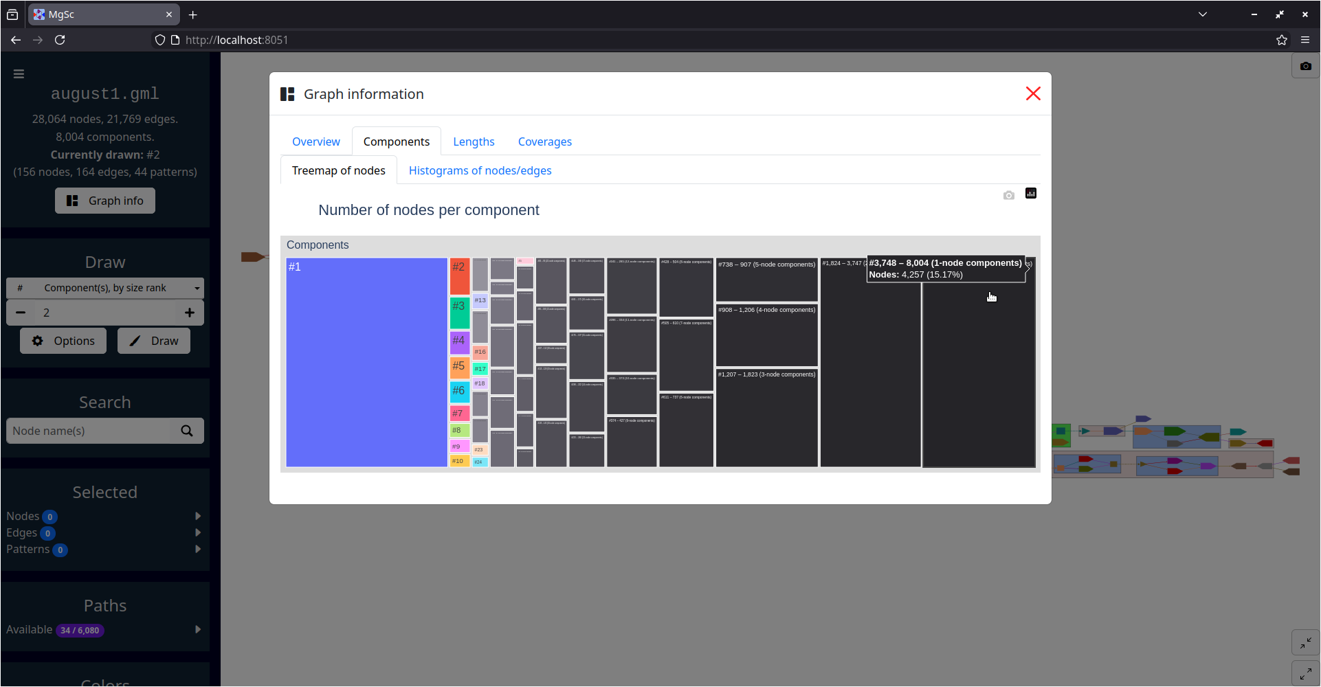
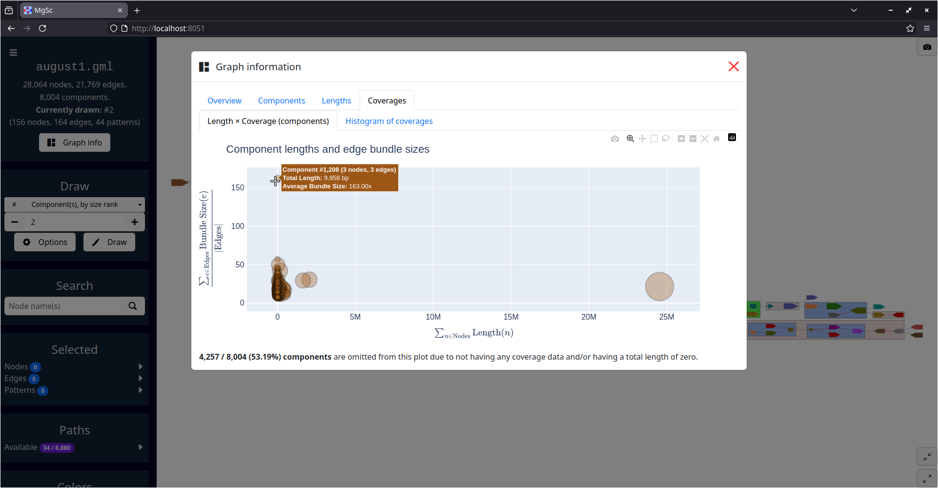
You can get a sense for the sizes of this graph's connected components by clicking the "Graph info" button in the left sidebar, then examining the charts in the "Components" tab.
Doing this for this example graph shows that the largest connected component in this graph (#1) contains over six thousand nodes. You can certainly draw this component in MetagenomeScope, but it will take a few seconds to lay out and draw. The resulting interface may also become a bit sluggish due to the amount of nodes and edges being drawn. (You could even draw the entire graph if you wanted to, as shown above! But it will be even more sluggish.)
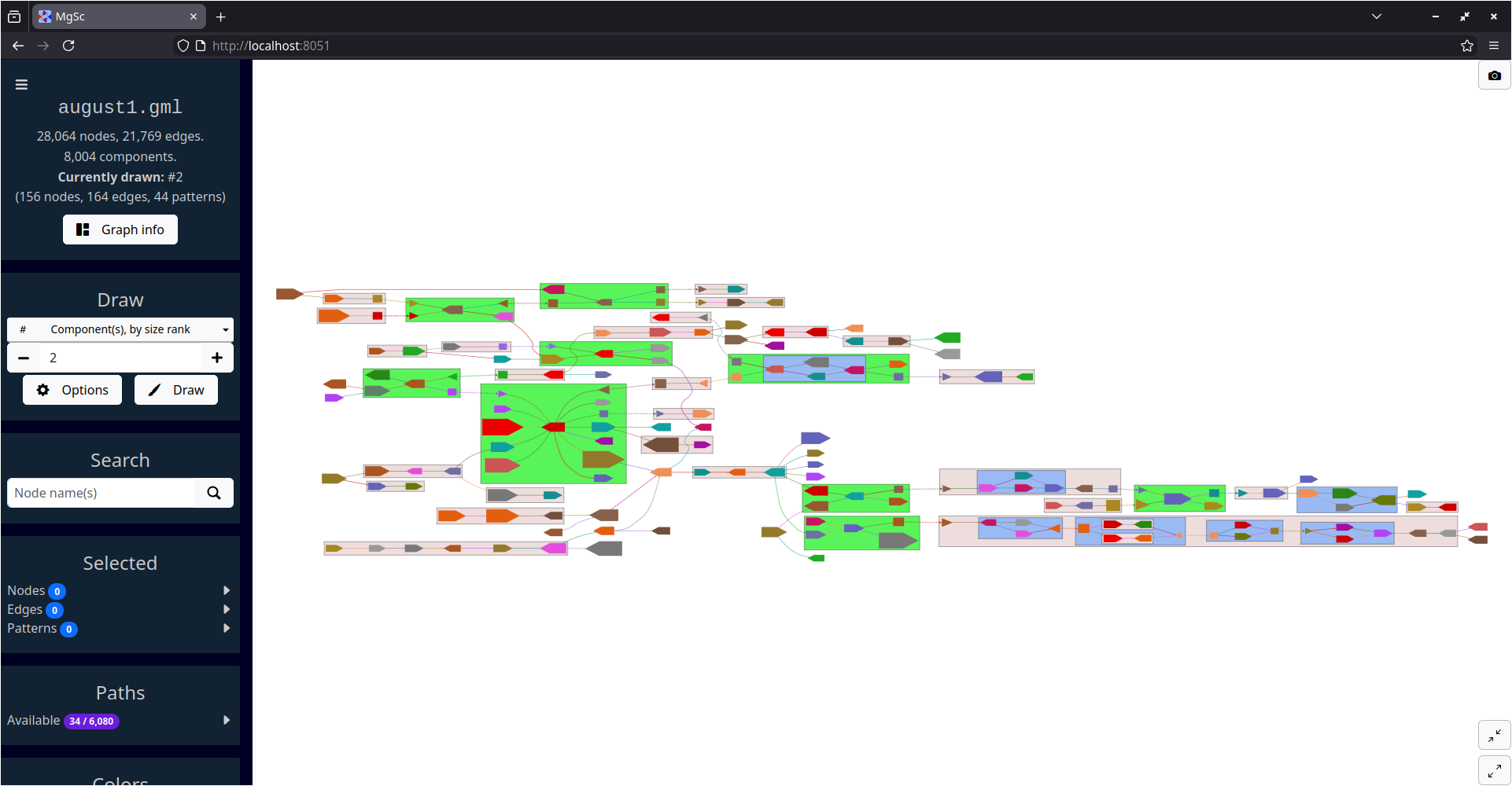
Looking at the treemap tells us that component #2 has far fewer nodes -- just 156. So, if we would like to draw some part of this graph (but skip the big hairball that is component #1), then it might make sense to start with component #2.
You can do this by replacing the 1 in the Draw section's text field with a 2, to indicate that we should draw component #2.
You can even draw a range of components, if you would like. Try typing 2-10 in the text field to draw all of these components at once!
You can also draw only a subregion of a larger component, using functionality inspired by Bandage. In the "Draw" section, change the "Component(s), by size rank" dropdown to the "Around certain node(s)" option, and then type in k99_38. Try increasing the distance and redrawing to see more and more of component #1!
See the metagenomescope/tests/input/
directory.
FAQ: How do you handle reverse-complementary nodes/edges?
The answer to this depends on the filetype of the graph you are using.
When MetagenomeScope reads in FASTG, DOT, and GML files, it assumes that these files explicitly describe all of the nodes and edges in the graph. So, let's say you give MetagenomeScope the following LJA-style DOT file:
digraph g {
  1 -> 2 [label="edge1 A99(2.4)"];
}
We will interpret this as a graph with two nodes (1, 2) and one edge
(1 -> 2).
However, for GFA and LastGraph files, MetagenomeScope cannot make the assumption that these files explicitly describe all of the nodes and edges in the graph. In these files, each declaration of a node / edge (in GFA parlance, "segment" / "link"; in LastGraph parlance, "node" / "arc") also declares this node / edge's reverse complement.
So, let's say you give MetagenomeScope the following GFA file (based on this example):
H	VN:Z:1.0
S	1	CGATGCAA
S	2	TGCAAAGTAC
L	1	+	2	+	5M
We will interpret this as a graph with four nodes (1, -1, 2, -2)
and two edges (1 -> 2, -2 -> -1). The presence of node X
"implies"
the existence of the reverse complement node -X, and the presence of edge
X -> Y "implies" the existence of the reverse complement edge -Y -> -X.
Interpreting the graph file in this way is analogous to
how "double mode" works in Bandage.
Based on the FASTG specification, shouldn't FASTG be an "implicit" instead of an "explicit" filetype?
It's complicated. The way I interpret the FASTG specification, each declaration of an edge sequence implicitly also declares this edge sequence's reverse complement; however, this is not the case for "adjacencies" between edge sequences.
In any case, the "dialect" of FASTG files produced by SPAdes and MEGAHIT lists edge sequences and their reverse complements (as well as adjacencies between edge sequences and their reverse complements) separately. Because of this, we consider FASTG to be an "explicit" filetype. (See pyfastg's documentation for details on how we handle reverse complements in FASTG files.)
FAQ: Why does my graph have node X and -X in the same component?
One common reason this happens is the presence of palindromic sequences: these can cause both a sequence and its reverse-complement to be connected to each other.
This often occurs with the big ("hairball") component in an assembly graph.
FAQ: What happens if an edge is its own reverse complement?
(This assumes that you have read the FAQ above on "How do you handle reverse-complementary nodes/edges?")
This can happen if an edge exists from X -> -X or from -X -> X in an
"implicit" graph file (GFA / LastGraph). Consider
this GFA file:
H	VN:Z:1.0
S	1	AAA
S	2	ACG
S	3	CAT
S	4	TTT
L	1	+	1	+	2M
L	2	+	2	-	2M
L	3	-	3	+	2M
L	4	-	4	-	2M
Since this GFA file contains four "link" lines, we might think at first that the corresponding graph
contains 4 × 2 = 8 edges. However, the graph only contains 6 unique
edges. This is because the reverse complement of 2 -> -2 is itself:
we know from above that X -> Y implies -Y -> -X, but
-(-2) -> -(2) is equal to 2 -> -2! The same goes for -3 -> 3:
-(3) -> -(-3) is equal to -3 -> 3.
Both of these edges "imply" themselves as their own reverse complements!
How do we handle this situation? As of writing, when MetagenomeScope visualizes these graphs it will only draw one copy of these "self-implying" edges. This matches the original visualization of this graph, and also matches Bandage's visualization of this GFA file.
Notably, since we assume that "explicit" graph files (FASTG / DOT / GML)
explicitly define all of the nodes and edges in their graph, MetagenomeScope doesn't do anything
special for this case for these files. (If your DOT file describes one edge
from X -> -X, then that's fine; if it describes two or more edges from X -> -X,
then that's also fine, and we'll visualize all of them.)
FAQ: What do you mean by a component's "size rank"?
Given a graph with N connected components: we sort these components by the number of nodes they contain, from high to low. We then assign each of these components a size rank, a number from 1 to N: the component with size rank #1 corresponds to the largest component, and the component with size rank #N corresponds to the smallest component.
Often, we only care about looking at individual components in a graph -- laying out and drawing the entire graph is not always a good idea when the graph is massive. Component size ranks are a nice way of formalizing this.
Some details about component size ranks, if you are interested:
-
The numbers shown in the treemap (accessible in the "Graph info" dialog) correspond exactly to component size ranks. So, the rectangle labelled #1 in the treemap corresponds to the largest component, the rectangle labelled #2 corresponds to the second-largest component, etc.
-
The exact component sorting functionality accounts for ties using a few criteria. After ordering components by their total numbers of nodes, we break ties using the number of (real) edges, the total sequence length, and the lexicographically smallest node / edge name in the component, among other criteria.
FAQ: Can my graphs have parallel edges?
Yes! MetagenomeScope supports
multigraphs. In general:
if your assembly graph file describes more than one edge from X -> Y, then
MetagenomeScope can visualize all of these "parallel" edges. (This is mostly
useful when visualizing de Bruijn graphs.)
The exact behavior of how we handle parallel edges is controlled by the
--rmdup command-line parameter; see below for details.
There are a lot of GFA files floating around out there that declare both
A -> B and -B -> -A on separate lines. This describes a graph where every
single edge has a duplicate parallel edge!
Bandage and Gfapy, among other tools, silently ignore these edges. To match
this behavior, the default value of --rmdup (gfaonly) means that -- for
GFA files only -- MetagenomeScope will detect and remove parallel edges.
Currently, the choice of
which edge(s) are removed is arbitrary.
After removing parallel edges, MetagenomeScope will log information about the number of removed edges on the command line.
If you are using a GFA file where parallel edges have meaning, you can specify
--rmdup n to tell MetagenomeScope to not remove parallel edges.
By default, MetagenomeScope will not remove parallel edges if the input graph was not a GFA file.
However, if you would like to force it to remove parallel edges, then you can
specify --rmdup y.
Notably, parallel edges not supported right now for FASTG files. I don't think I've ever seen any FASTG files that have parallel edges, so I don't think this is a big priority, but I guess please let me know if you would like us to add support for it.
FAQ: What filetype should I use for de Bruijn graphs?
If you are visualizing output from LJA or Flye, you may want to use a DOT file instead of a GFA / FASTG file as input.
This is because GFA and FASTG are not ideal for representing graphs in which sequences are stored on edges rather than nodes (i.e. de Bruijn / repeat graphs). The DOT files output by Flye and LJA should contain the original structure of these graphs (in which edges and nodes in the visualization actually correspond to edges and nodes in the original graph, respectively); the GFA / FASTG files usually represent altered versions in which nodes and edges have been swapped, which is not always an ideal representation (especially if you are doing something where you really care about the structure of the original graph).
That being said, please note that -- if you are using an assembler that outputs graphs in different filetypes -- these files may have additional differences beyond the usual filetype differences. For example, Flye's GFA and DOT files can have slightly different coverages, since Flye produces them at different times in its pipeline.
FAQ: How do you handle E-lines in GFA 2 files?
We only visualize E-line edges that are classified as
"dovetails." That is, edges
that connect the ends of two nodes -- for example:
     | |
------->
     ------->
Note that our rules for classifying dovetail edges are currently somewhat stricter than those outlined in the GFA 2 specification. See this issue for details.
FAQ: How do you handle O-lines in GFA 2 files?
I'm so glad you asked! Although I am doubtful that anybody is actually asking this question, so maybe you are not a real person.
ANYWAY so okay here's the deal. In GFA 1 files, paths (P-lines) are relatively simple -- they can only
contain segments. So P-lines are refreshingly easy to reason about.
In GFA 2 files, however, paths (O-lines) can contain other things besides segments -- they can also contain
edges, or even other paths! There are some interesting considerations this flexibility brings up.
There is no guarantee that O-lines are given in any particular order, so you can have dreadful
situations where a path with ID B says that it contains a path with ID A (which is
defined in a later line in the file).
We handle this by -- after scanning through the entire GFA file -- creating a directed graph, where each
edge A -> B indicates that path B contains path A. We then use NetworkX to find a
topological ordering
of the nodes (paths) in this graph, and record paths (in terms of just their child segments
and nothing else) in this order. Using the topological ordering ensures that, when it is time
to record a path, we already know the exact contents of the paths that it contains -- so we can
safely "expand" the child paths.
If you really wanted to make our jobs hard, you could create a GFA file with cycles: where path
B contains A which contains C which contains B (or something like that).
If we detect this kind of situation, we will raise an error (because like how should we even handle this...?)
In GFA 2, edges can optionally have IDs. You can refer to these edge IDs on an O-line in GFA 2.
Currently, MetagenomeScope assumes that all paths loaded from GFA files will only contain nodes -- not a mixture of nodes and edges. Thus, when MetagenomeScope notices that a GFA 2 path contains an edge, it converts this edge into the 2-tuple (source, target) in the path.
Later, we "expand" these 2-tuples (turning the path into just a basic list of segment IDs) according to the following logic.
- If "source" is not already given as the previous entry in the path, then we add it to the path.
- If "target" is not already given as the next entry in the path (as a segment), then we add it to the path.
I think this should mostly match how other GFA 2 parsers (e.g. Gfapy) handle these kinds of mixed paths.
Note that if your GFA 2 file describes a multigraph (i.e. it has parallel edges, and you specified edge-paths in order to disambiguate which specific edges the path traverses) then this process will inherently cause some ambiguity. If you have strong opinions about this, please feel free to file an issue so we can discuss.
FAQ: My graph is a DOT file from LJA that does not have edge IDs. Can I still create a "paths" file for it?
Yes!
Some background: in some older LJA graphs, edges do not have explicitly set IDs.
MetagenomeScope will detect this, and automatically create edge IDs
in the format SOURCE → TARGET (FIRST NT). (That is, using the literal right arrow
unicode symbol -- i.e. U+2192.)
So, if you want to specify paths through these graphs that do not have
edge IDs, then: you can prepare your AGP (-a) or TSV (-t) file as normal,
but just refer to edges' IDs in this format. (Make sure to label the orientation
of each of these edge IDs as +, even if it contains negative-strand node(s).)
Here is an example of how you could do this:
FAQ: How can I run the pattern decomposition process programmatically?
Creating a metagenomescope.graph.AssemblyGraph object will automatically run the decomposition process:
>>> from metagenomescope.graph import AssemblyGraph
>>> ag = AssemblyGraph("graph.gfa")  # replace with your graph's filepath
At this point:
-
The "decomposed graph" (where patterns are collapsed into nodes) is represented by
ag.decomposed_graph(a NetworkXMultiDiGraph). -
The "true graph" (i.e. with all patterns fully uncollapsed, revealing all "original" nodes and edges) is represented by
ag.graph(also a NetworkXMultiDiGraph)- Note that this graph will still include split nodes and fake edges, if any remain after the decomposition process.
-
All nodes, edges, and patterns will have unique integer IDs. These IDs can be used to look up information about nodes, edges, and patterns in the
ag.nodeid2obj,ag.edgeid2obj, andag.pattid2objdictionaries, respectively.
Some examples of things you can do with the AssemblyGraph object:
>>> from metagenomescope.graph import AssemblyGraph
>>> ag = AssemblyGraph("metagenomescope/tests/input/E_coli_LastGraph")
>>> # How may connected components are in the graph?
>>> import networkx as nx
>>> len(list(nx.weakly_connected_components(ag.graph)))
61
>>> # Inspect node / edge / pattern MetagenomeScope objects
>>> ag.nodeid2obj
{0: Node 0 (name: 1),
 1: Node 1 (name: -1),
 2: Node 2 (name: 2),
 ...}
>>> ag.edgeid2obj
{558: Edge 558 (orig: 0 -> 244; new: 0 -> 244; dec: 0 -> 1421),
 559: Edge 559 (orig: 1 -> 342; new: 1 -> 342; dec: 1527 -> 342),
 560: Edge 560 (orig: 2 -> 477; new: 2 -> 477; dec: 2 -> 477),
 ...}
>>> ag.pattid2obj
{1222: bubble1222 containing nodes [33, 283, 395, 39] from [33] to [39],
 1227: bubble1227 containing nodes [34, 76, 382, 303] from [34] to [76],
 1232: bubble1232 containing nodes [40, 43, 35, 501] from [35] to [43],
 ...}
>>> # Go through just the bubble patterns
>>> ag.bubbles
[bubble1222 containing nodes [33, 283, 395, 39] from [33] to [39],
 bubble1227 containing nodes [34, 76, 382, 303] from [34] to [76],
 bubble1232 containing nodes [40, 43, 35, 501] from [35] to [43],
 ...]
>>> # Look up a node by name (if a node was split, this will list both halves)
>>> ag.nodename2objs
defaultdict(<class 'list'>,
            {'1': [Node 0 (name: 1)],
             '-1': [Node 1 (name: -1)],
             '2': [Node 2 (name: 2)],
             ...
             '40-R': [Node 78 (name: 40-R)],
             '40': [Node 78 (name: 40-R), Node 1259 (name: 40-L)],
             '40-L': [Node 1259 (name: 40-L)],
             ...})
>>> # Examine split nodes
>>> for n in ag.nodeid2obj.values():
...     if n.split is not None:
...         print(n)
Node 32 (name: 17-L)
Node 33 (name: -17-R)
Node 34 (name: 18-R)
...
>>> # Distinguish fake from real edges
>>> for e in ag.edgeid2obj.values():
...     print(e, e.is_fake)
Edge 558 (orig: 0 -> 244; new: 0 -> 244; dec: 0 -> 1421) False
Edge 559 (orig: 1 -> 342; new: 1 -> 342; dec: 1527 -> 342) False
...
Edge*1634 (orig: 348 -> 1633; new: 348 -> 1633; dec: 1628 -> 1666) True
Edge*1639 (orig: 1638 -> 451; new: 1638 -> 451; dec: 1671 -> 1635) True
This interface should remain relatively stable, although I may change things slightly as development continues. If you have any questions, please reach out.
FAQ: Okay just kidding I actually don't care about patterns. Can I load the graph without running the pattern decomposition process at all?
You sure ask a lot of questions!
Anyway, the answer is yes.
Maybe your graph is super large and running decomposition takes too long, or maybe you just want
to look at the structure of the graph without having to even think about split nodes and fake edges.
In any case: you can tell MetagenomeScope to skip the pattern decomposition stuff by setting
run_decomposition=False when you initialize the AssemblyGraph object:
>>> from metagenomescope.graph import AssemblyGraph
>>> ag = AssemblyGraph("graph.gfa", run_decomposition=False)
Now you can mess around with the unmodified ag.graph NetworkX object to your heart's content.
If you wanted to, I guess you could use MetagenomeScope as an intermediate assembly graph parser in this way. (I mean, that wasn't really why we wrote this software in the first place, but I'm not your mom.)
FAQ: What's the biggest possible graph I can visualize?
We're still figuring that out. There are a couple steps that can be time-consuming for big graphs, including:
-
Processing the graph.
- Because we (currently) store the entire graph in memory, massive graphs -- with millions of nodes / edges -- can become impractical to load on low-memory systems.
-
Decomposing the graph into patterns.
- I've done some work on optimizing this; the first phase (finding bubbles/bulges, chains, and cyclic chains) is generally slower than the second phase (finding frayed ropes and bipartites).
-
Laying out the graph (or some part of it).
-
When you get to the order of, say, thousands of nodes, laying out a connected component of the graph will probably become somewhat slow (especially if you select the
Lay out patterns recursivelyoption in the draw options dialog). -
To my understanding, a big factor here is the ratio of nodes to edges: when there are many more edges than nodes in a component (indicating a very densely connected structure), Graphviz has to do a lot of work to position things properly. In such cases, using the sfdp layout algorithm will probably speed things up.
-
-
Drawing the graph's elements in the browser.
-
Cytoscape.js has a lot of optimizations built-in, but I think there are some inherent limitations of drawing using a HTML canvas.
-
With graphs containing thousands of nodes, interaction (e.g. zooming, panning) starts to feel a bit sluggish.
-
See the "Large graph" section under "Example datasets" above for some tips for working with large graphs.
FAQ: I want to benchmark how long this tool takes to run. How can I do that?
Make sure to run mgsc with the --verbose flag. This will log pretty detailed information about
the various steps MetagenomeScope is doing, and the times at which they take place (e.g. when each
phase of pattern decomposition starts and ends, when laying out a region of the graph starts and ends, ...)
Eventually I would like to show more of this information in the browser (and/or summarize it in an easy-to-parse text file?) -- if you have opinions about this, feel free to open an issue.
-
Edge flattening: In certain cases, we may be unable to draw an edge with complex control points. Usually this happens when Cytoscape.js does not accept the control points Graphviz produced for an edge, but sometimes Graphviz will be unable to create control points for an edge in the first place. (Or sometimes an edge will get routed into the middle of nowhere...)
In any case: MetagenomeScope will detect these kinds of edges and "flatten" them into simple Bezier edges (usually straight lines). This way, we can at least draw something for each edge in the graph.
See CONTRIBUTING.md.
See CHANGELOG.md.
MetagenomeScope is licensed under the GNU GPL, version 3.
MetagenomeScope's code is distributed with
Bootstrap,
Bootstrap Icons,
Cytoscape.js,
layout-base,
cose-base,
cytoscape-fcose,
dagre,
cytoscape-dagre,
and
cytoscape-svg.
Please see the metagenomescope/assets/vendor/licenses/ directory for copies of these tools' licenses.
Thanks to various people in the Pop, Knight, and Pevzner Labs over the years for their kind feedback and helpful suggestions.
Thanks also to the developers of the many excellent open-source software packages used by MetagenomeScope. In particular, Graphviz (graph layout), Cytoscape.js (interactive graph drawing), and Dash (application framework) have been extremely helpful tools throughout the development of this project.
Some of MetagenomeScope's software tests use data from other places. Please see the
metagenomescope/tests/input/
directory's README for a list of acknowledgements.
Please open a GitHub issue if you have any questions or suggestions.