Module 2

2.1 2D Convolution

Convolution is a simple mathematical operation that is fundamental to many common image processing operators [1]. The idea behind convolution is to study how one function when mapped with another function brings out a new modified function. But that's a lot of words for what it really is in practice (when working with images).

We can think of an image as a 2Dimensional matrix containing pixel color values in the range of 0 to 255.

Now, realize that this matrix is the first function of our equation. Consequently, we need the second function that will map our first function (our image). This second function is known as kernels. In image processing; kernel, filter, convolution matrix, or mask is a small matrix used for blurring, sharpening, embossing, edge detection, and more [1, 2, 3].

Design of kernels is based on high levels mathematics. There, now that we have our two functions, you may wonder how they operate so that one maps to the other and we get the new function (a blurred image or with the edges highlighted or sharpened, etc.), well instead of trying to explain it, see for yourself:

Simple, at the beginning the origin of the kernel will coincide with the corner of our image (in this case), an element-wise multiplication is computed, then all the values of this multiplication are added, and the result will be the corner of the new image. Then the kernel origin will iterate through the whole image and we get our new image smoothed or sharpened, etc.

Padding

As you could see in the animation above, when the kernel is at the edges of the image, it had values that did not match any in the image and these were multiplied by some numbers. Those numbers that 'extend' the image are called padding. Padding involves adding extra pixels around the border of the image before convolution [4].

There are several types of paddings used in deep learning (blue maps are inputs, and cyan maps are outputs) [5]:

• Valid: This type of padding can be considered as no padding. Here the output image is smaller than the input image.

• Same: Here, padding is added to the input image such that the size of the output image is the same as the input image (this is the type of padding that has the first convolution animation we saw).

• Full: Unlike the previous two types that reduce or maintain the image size, this one increases it. This can be achieved with a suitable padding.

Additionally, you can also vary the values with which the padding is filled, some of these variations are: with zeros, with a constant, with a reflection, with a replication or circularly, see it in detail here. Here you may also notice that the amount of padding that is added horizontally should not be strictly the same as vertically. There are cases where more is added in one direction than in the other.

If you want to study a little bit in depth why padding is used, I recommend you to check the following resources [6, 7].

Kernel Size

Basically, the height and width that our filter/kernel will have. The following are the most commonly used sizes.

Stride

The stride is a parameter of the convolution operation that refers to the number of pixels by which the filter matrix moves across the input matrix. When the stride is 1, the filter moves across the input matrix 1 pixel at a time. When the stride is 2, the filter jumps 2 pixels at a time as we slide it around. And so on [8]. It looks like this:

As you may have noticed, the stride can be configured to be applied both vertically and horizontally. One note to mention is that the convolution is not computed if the kernel is NOT fully contained within the image.

Let's combine them

At the end you will have several parameters (there are more) that you can configure to your liking. For example, in Pytorch these parameters are called as follows.

torch.nn.Conv2d(in_channels, out_channels, kernel_size, stride=1, padding=0, dilation=1, groups=1, bias=True, padding_mode='zeros', device=None, dtype=None)

• kernel_size: controls the filter size
• stride: controls the stride for the cross-correlation, a single number or a tuple.
• padding: controls the amount of padding applied to the input. It can be either a string {‘valid’, ‘same’} or an int / a tuple of ints giving the amount of implicit padding applied on both sides.
• padding_mode: controls with which method we are going to fill the padding

2.2 Convolutions in Neural Networks

As you are curious you may have wondered what in_channels, out_channels, dilation, groups, bias mean (device and dtype are related to the hardware and data type with which the computation will be performed, so we will not deal with them). So, I would like to welcome you to true convolution, the one that allows us to classify puppies in images, tell us in which pixels a person is located, detect objects and even classify breast cancer ;).

I strongly recommend you to watch the explanations of the following channel, they are extremely valuable to understand these concepts.

In channels and Out channels

The input channels are the number of matrices that represent our image, for example, in a grayscale image only one matrix is needed (in_channels = 1), this is the case of the images that we were seeing in the 2D Convolution section. But in case of an RGB image we need three (in_channels = 3) or in case of a spectral image we need several.

And the output channels are the number of filters through which we will convolve our input channels. These filters will have the same depth as the input channels. For example, if we create our convolution with the following parameters:

torch.nn.Conv2d(in_channels=3, out_channels=1, kernel_size=3, stride=1, padding='valid')

We will have one (1) filter of size 3x3 with three (3) depth channels that will convolve with our input image that also has three (3) depth channels, visually it will look like this:

In the gif, what you see shaded in the image is the filter iterating through each input channel. Then, each cube that appears is the result of the element-wise multiplication between each input channel and its corresponding filter channel. And at this moment you see that three (3) channels come out of the convolution, and we put that we wanted only one (out_channels=1), so, what happens now is to add those three channels to end up with only one.

Thanks to the following source for the images, I invite you to check it out.

Bias

Finally, then there’s the bias term. The way the bias term works here is that each output filter has one bias term. The bias gets added to the output channel so far to produce the final output channel [9].

An example both visually and mathematically of what is going on that I like is the following. In this example we have in_channels = 3 (any RGB image), with a particular padding and we are convolving it with one (1) filter.

Dilation

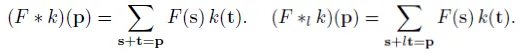
The left one is the standard convolution. The right one is the dilated convolution. We can see that at the summation, it is s+lt=p that we will skip some points during convolution [10]. Don't worry, you don't have to be a math major to know what the equation does, visually it's very easy to understand:

Standard Convolution (l=1)	Dilated Convolution (l=2)

On the left we have the standard convolution l=1 and on the right we have an example of dilated convolution when l=2 (same as torch.nn.Conv2d(in_channels=1, out_channels=1, kernel_size=3, stride=1, padding=0, dilation=2)). We can see that the receptive field is larger compared to the standard one.

The above figure shows more examples about the receptive field. What is this useful for? Well, according to Yu and Koltun (2015) dilated convolutions support exponentially expanding receptive fields without losing resolution or coverage. They developed a new convolutional network module (in 2015) based on dilated convolutions for semantic segmentation and increased the accuracy of state-of-the-art.

Groups

The idea here is to 'separate' the number of channels that the filters will have in N groups (up to the maximum number of input channels). Honestly, I would try to explain textually how it works, but the following video does it better, so I'll just leave the gifs he uses to have them at hand.

1 Group	2 Groups

To contribute something (because the video is great), the two-group convolution in code would look like this:

torch.nn.Conv2d(in_channels=8, out_channels=8, kernel_size=3, stride=1, padding=0, dilation=1, groups=2)

The main purpose of doing this is to reduce the computational complexity (in the Encoder section we will study why) of performing such deep operations.

Depthwise Convolution

What we do here is to use as many groups as there are channels in the input. Again, thanks to Animated AI for making the following animation:

torch.nn.Conv2d(in_channels=8, out_channels=8, kernel_size=3, stride=1, padding=0, dilation=1, groups=8)

It is as if we had a grayscale image (a single channel) and convolved it with one (1) filter, that for eight times and at the end we concatenated everything. But if we do this repeatedly we will lose all the information that is related between the channels (at the depth level).

Depthwise-Separable Convolution

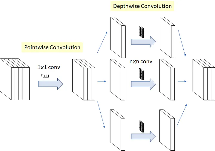
Pointwise Convolution: To remedy the Depthwise Convolution problem and use as little computation as possible, one by one or pointwise convolutions are applied to map correlations at depth level. In code it looks like this (check the kernel_size and groups):

torch.nn.Conv2d(in_channels=8, out_channels=8, kernel_size=1, stride=1, padding=0, dilation=1, groups=1)

If we apply the two types of convolution one after the other, it will look like this (i recommend you to watch the video to understand it):

Here is the code:

torch.nn.Sequential(
  torch.nn.Conv2d(in_channels=8, out_channels=8, kernel_size=3, stride=1, padding=1, groups=8, bias=False), # depthwise
  torch.nn.Conv2d(in_channels=8, out_channels=8, kernel_size=1, stride=1, padding=0, groups=1, bias=False) # pointwise
)

The intuition behind this is that cross-channel correlations (at the depth level) and spatial correlations are sufficiently decoupled that it is preferable not to map them at the same time [11].

Deformable

This type of convolution gained popularity in 'Deformable Convolutional Networks' a paper published by Dai et al. (2017). They assure that a key issue with traditional convolutions is their inability to adapt to geometric variations and transformations. Using fixed geometric structures [12].

One way to attack this problem is to perform transformations to the input images (data augmentation) but they explored something different, instead of transforming the inputs, why not transform the convolutions. So what are deformable convolutions? Deformable convolutions allows the filter to dynamically adjust its sampling locations with learnable offsets so that a better spatial relationship of the input data may be modelled.

Regular sampling grid (green points) of standard convolution	Deformed sampling locations (dark blue points) with augmented offsets (light blue arrows) in deformable convolution	Special case of deformable convolution	Special case of deformable convolution

How does this work? First we have to go over standard convolution, so imagine the region that a filter looks at as a grid. To each pixel, we are going to put some coordinates (offset=0). Standard convolution multiplies each filter weight with its corresponding coordinate (offset=0) in the field we are looking at in the image.

Field of the image that the filter is looking at as a grid	Standard convolution modeled in a different way

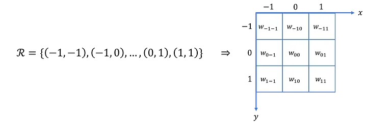
In deformable convolutions, we introduce a grid R that is augmented by offsets $\Delta p_{n}$. This essentially means that the grid R becomes irregular and grid boxes shift ever so slightly. Understand that what is shifted is not the filter, it is the fields that the filter looks at, specifically, the pixel value by which the filter weights are multiplied.

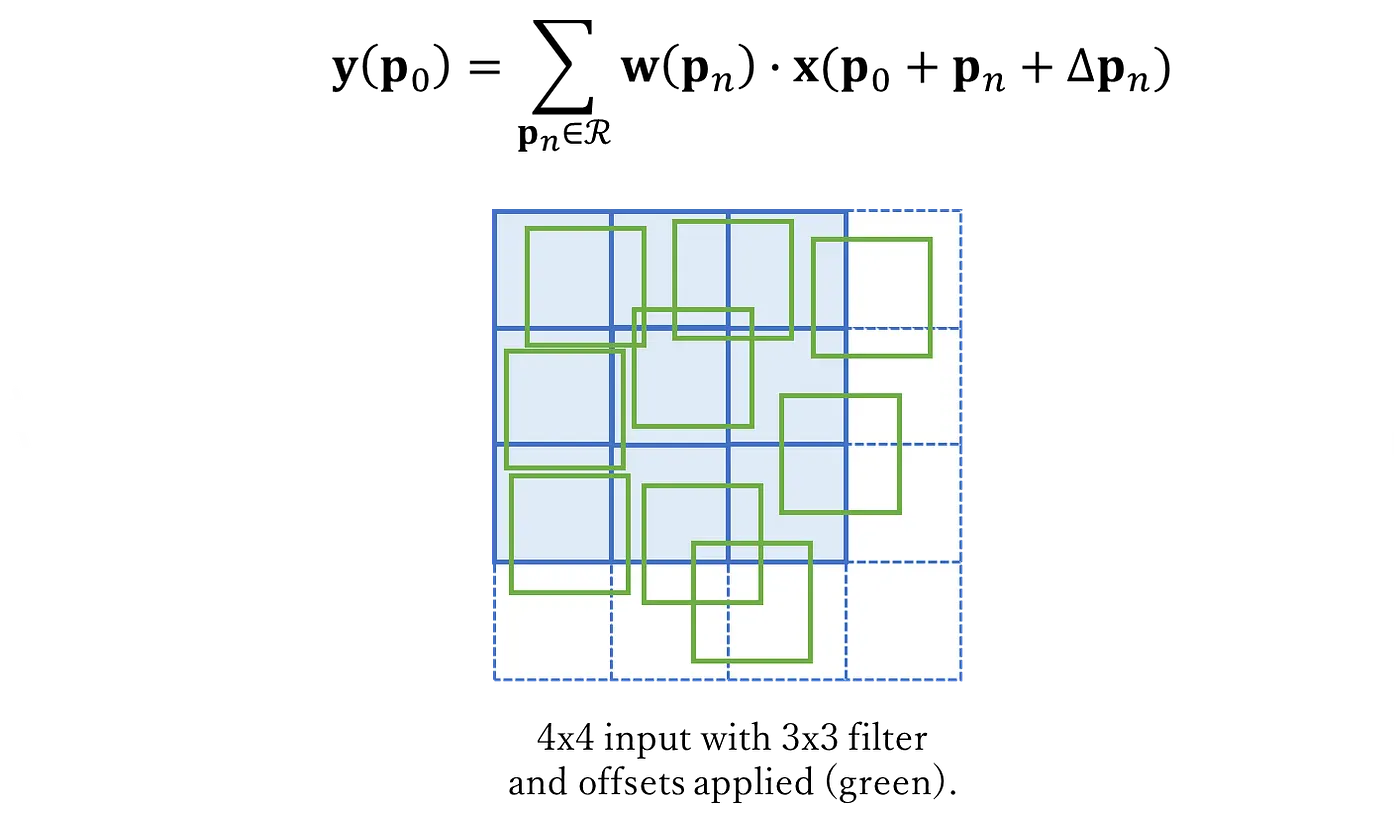
The numerical value of a pixel results from the combination (by means of bilinear interpolation) of several nearby pixels, depending on the offset applied to it. Let's see how:

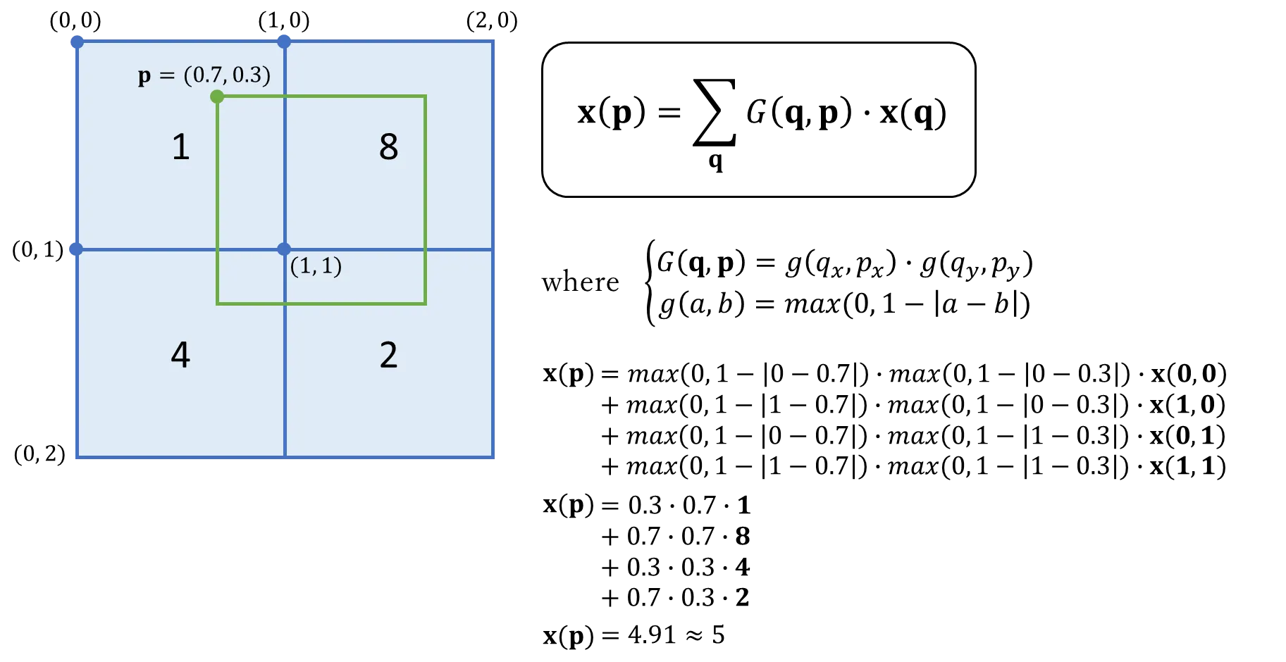
Brief explanation about the example (stolen from here):

• In the image above, there are four pixels with their values shown.
• In green, an offset pixel p with a fractional location is shown. Note that p's original pixel location is not important as bilinear interpolation depends only on surrounding pixels.
• We must use the same reference point for each pixel when measuring the offset distance between pixels. In this example, I chose the top left-hand corner of each pixel (other points such as top right, bottom left or centre, could have also been chosen).
• $\mathbf{G(q, p) = 0}$ for all pixels not in the offset pixel’s immediate surrounding. This is because $\mathbf{g(a, b) = max(0, 1 - |a - b|) = 0 as 1 - |a - b| < 0}$ for all pixels q further that one pixel length from the offset pixel p. This is why we only use four pixels for bilinear interpolation.
• Substituting all the values gives us an approximate pixel value of 5, which makes sense if we look at it visually.

The visual implementation looks like this:

How is this implemented in code? Don't worry (fortunately) they already did, if you want to experiment with this type of convolution you can find its implementation in Pytorch:

torchvision.ops.deform_conv2d(input: Tensor, offset: Tensor, weight: Tensor, bias: Optional[Tensor] = None, stride: Tuple[int, int] = (1, 1), padding: Tuple[int, int] = (0, 0), dilation: Tuple[int, int] = (1, 1), mask: Optional[Tensor] = None)

2.3 Pooling

All that this layer does is reduce the amount of computing power needed to process the data. This is accomplished by further reducing the size of the featured matrix. In this layer, we are attempting to isolate the most important properties of a small neighborhood [13].

There are two types of widely used pooling in CNN layer:

• Max Pooling: is merely a rule that takes the maximum of a region, and it is useful for moving forward with the most significant aspects of a picture. The max pooling algorithm chooses the pixels in an image that are the brightest. It comes in handy in situations in which the background of the image is dark and we are only interested in the pixels that are bright in the image.

• Average Pooling: Unlike Max Pooling, which removes all non-essential parts from a block or pool, Average Pooling keeps significant information about the “less important” aspects. However, unlike Maximizing your pooling, Average Pooling doesn’t simply discard them. Any situation in which this kind of information might be helpful could benefit from knowing this information.

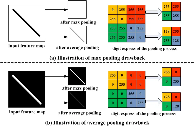Visual example of both types	Comparison of how they affect

Images are taken from here. Both are also implemented in Pytorch (max, average)! Those in the GIF on the left are implemented as follows:

torch.nn.MaxPool2d(kernel_size=2, stride=2, padding=0, dilation=1, return_indices=False, ceil_mode=False)
torch.nn.AvgPool2d(kernel_size=2, stride=2, padding=0, dilation=1, return_indices=False, ceil_mode=False)

Global Pooling Layers

Global Pooling Layers often replace the classifier’s fully connected or Flatten layer. The model instead ends with a convolutional layer that produces as many feature maps as there are target classes and performs global average pooling on each of the feature maps to combine each feature map into a single value [14].

In the image, 'd' is equal to the number of channels. The word 'GAP' in the image refers to Global Average Pooling, although it can also be implemented with Max, i.e. 'GMP'. As usual, they are also implemented in Pytorch! (GAP, GMP).

2.4 Encoder

Summary: an encoder is an architecture that allows us to encode or process the input data (images) and transform it into a different representation.

Play with a demo

First I would like you to start playing with the following simulator, it is quite good and maybe it will help you to better understand the concepts that we reviewed in the previous sections, if you do not understand it at first you can see the following tutorial that is at the end of its page.

History

Let's start with a bit of history. The first widely recognized convolutional neural network (CNN) that (to my knowledge) was designed is LeNet, created by Yann LeCun in the late 1980s. It was one of the earliest neural networks to use convolution and pooling layers, paving the way for modern deep learning applications in image recognition.

I am sure that after having reviewed the initial concepts, you are not so lost when looking at the architecture. Maybe you are wondering what are the feature maps. Feature map and activation map mean exactly the same thing. It is called an activation map because it is a mapping that corresponds to the activation of different parts of the image, and also a feature map because it is also a mapping of where a certain kind of feature is found in the image [15].

If we look again at the animation that I like so much of the convolution, exactly the feature maps are that three-dimensional aquamarine cube through which the filters will be convolved. The same way, the rainbow cube that comes out after applying the convolutions is a feature map.

As you can see from the LeNet architecture and the convolution animation, as convolutions are made, the dimension of the features (i.e. the number of channels) increases while the height and width of the features decreases. In other words, what is happening there is that the image information is being encoded.

LeNet's main limitations were due to computational power, as it relied on CPUs for training. This restricted its ability to process larger datasets or complex images efficiently. But the Deep Learning community did not give up and in 2012 Alex Krizhevsky et al. designed an architecture quite similar to LeNet, but with the difference that its computations were computed on 2 GPUs (yes!, parallelization). This architecture is called AlexNet and was a breakthrough that used convolutional nets to almost halve the error rate for object recognition, and precipitated the rapid adoption of deep learning by the computer vision community [16].

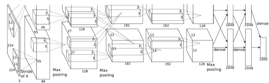
You may think that the image was cropped, but no, this is how it was originally included in the paper. You can find an implementation from scratch in Pytorch here, an explanation here and even a video in Spanish here.

We need going deeper

There are also significant differences between AlexNet and LeNet. First, AlexNet is much deeper than the comparatively small LeNet-5. AlexNet consists of eight layers: five convolutional layers, two fully connected hidden layers, and one fully connected output layer. Second, AlexNet used the ReLU instead of the sigmoid as its activation function [17].

That's when VGG appears, Simonyan and Zisserman (2014) published the paper "Very Deep Convolutional Networks for Large-Scale Image Recognition".

Our main contribution is a thorough evaluation of networks of increasing depth using an architecture with very small (3x3) convolution filters, which shows that a significant improvement on the prior-art configurations can be achieved by pushing the depth to 16-19 weight layers.

You may wonder why this architecture is important, well, basically they showed that depth of representation is beneficial for classification accuracy, and that state-of-the-art performance on the ImageNet challenge dataset can be achieved using a conventional ConvNet architecture (LeCun et al., 1989; Krizhevsky et al., 2012) with substantially greater depth.

Our results yet again confirm the importance of depth in visual representations.

And I want you to keep the phrase 'depth in visual representations' because it's the key. Depth in visual representations is another way of saying 'encoded information' or 'high level features'. The features found in deeper layers of a CNN are high level features because they have a lot of information at the image depth level, but very low information at the spatial level, while the features found in initial layers are low level features because they have very low information at the depth level, but are quite rich with spatial information.

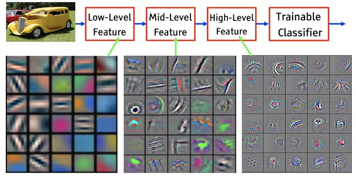
• Low-level/Primitive features: extract edges & lines of the images. These are primitive feature extractors (filters) which pick up minor details of the image like lines , curves & dots.
• Higher-Level features: depict complex patterns which resemble parts of objects in images which tend to be a unique trait of for that class(object), which contributes to classification score for that class as well.

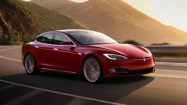
Tesla model S	Low level features	Higher level features

Here, low level feature maps are from the initial layers of VGG16 network trained on ImageNet dataset. The primitive features horizontal, vertical & 45⁰ lines help depict the shape of the car’s body. And high feature maps are from the higher layers of VGG16, the images might be difficult to comprehend, but by looking closer at the image on the right we notice details such as the windows, the tires etc. [18].

In the following link you can find an explanation of the implementation of this network from scratch in Pytorch.

To conclude, an encoder is an architecture that allows us to encode or process the input data (images) and transform it into a different representation.

The problem with Going Deeper with Convolutions

Computational cost

Something I haven't told you is that as the number of layers in a convolutional neural network increases, so does the number of parameters to learn, and that translates into higher computational cost and longer training times (and life is too short to just watch a network train).

LeNet-5, designed for digit recognition, had about 60,000 parameters, making it a relatively small network. AlexNet, had 62 million parameters. VGG-16, significantly increased the number of parameters to 138 million. The images in the following table were taken from here and here.

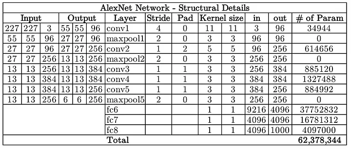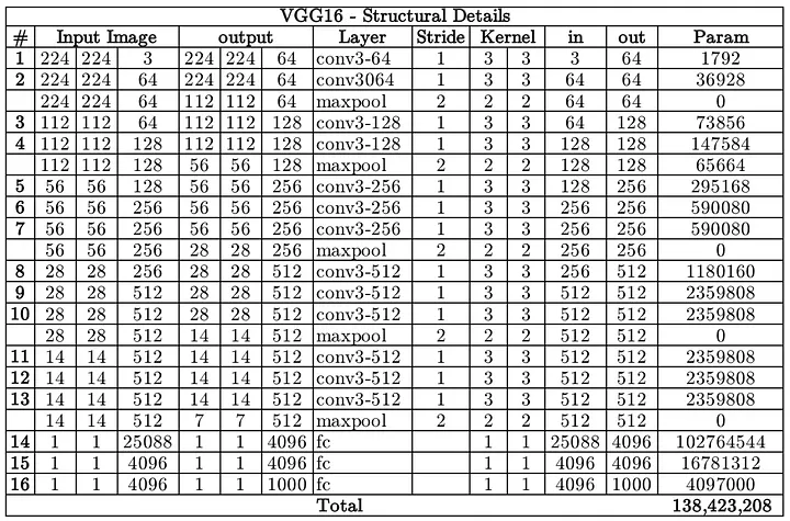LeNet-5 number of parameters	AlexNet number of parameters	VGG-16 number of parameters

This is when a paper literally called “Going Deeper with Convolutions” (Szegedy et al., 2014) appears. A paper in which they studied how to reduce the computational cost of CNNs without reducing the depth of the networks. The basic idea is to apply a 1x1 convolution before applying any other operation (3x3, 5x5 or pooling) and this reduces by a factor of 10 the computational cost, you can watch the following video where Andrew Ng explains it very well.

The Pytorch implementation of this network can be found in our repository 🥳!

A little later, Chollet (2016) proposed an extreme version of Inception V3, called Xception, which applied a stronger hypothesis than Inception and used techniques such as residual connections.

Would it be reasonable to make a much stronger hypothesis than the Inception hypothesis, and assume that cross-channel correlations and spatial correlations can be mapped completely separately?

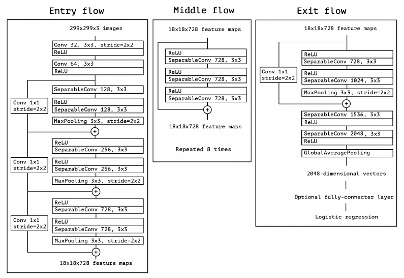Xception module	The Xception architecture

The Pytorch implementation of this network can also be found in our repository 🥳!

Vanishing/Exploding Gradient

When I talked about Xception I mentioned residual connections. For you to understand what they are first you must understand what they are for. In this video, Andrew Ng explains it much better.

When a network becomes deeper, gradients, which are used to update weights by algorithms such as SGD or Adam, can get so small (vanishing) that layers near the input do not learn properly, or they can get too large (exploding), leading to unstable updates. Residual connections allow information to skip some layers, improving gradient flow and ensuring that all layers can learn. This helps prevent gradients from disappearing or exploding, allowing for efficient training of deep networks such as Xception.

Residual connections were first introduced in the computer vision community by He et al. (2015) in ResNet. You can find an explanation of the paper and its implementation in Pytorch and in Spanish here, thanks Pepe Cantoral.

2.5 Decoder

You might have already explored how convolutions help us extract features from images. But what if we need to generate or reconstruct images instead of just analyzing them? This is where decoders come into play, especially in tasks like image segmentation and generative models (e.g., GANs).

In this section, we'll dive into the fundamental operations used in decoders: upsampling, transposed convolutions, and pixel shuffle. These are the building blocks for upscaling feature maps back into images.

Upsampling

When decoding, one of the most important tasks is to increase the size of our feature maps. Upsampling is exactly that — it's the process of increasing the spatial dimensions of a feature map. The following images were taken from here and here.

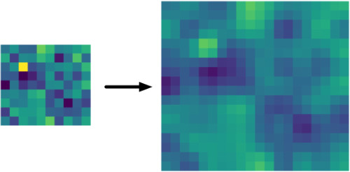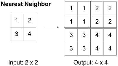Bilinear Upsampling	Upsampling with Nearest Neighbor aka Unpooling

In PyTorch, upsampling is built into the torch.nn.Upsample class representing a layer called Upsample that can be added to your neural network. The Upsample layer is made available in the following way:

torch.nn.Upsample(size=None, scale_factor=None, mode='nearest', align_corners=None, recompute_scale_factor=None)

These attributes can be configured:

• With size, the target output size can be represented. For example, if you have a 28 x 28 pixel image you wish to upsample to 56 x 56 pixels, you specify size=(56, 56).
• If you don't use size, you can also specify a scale_factor, which scales the inputs.
• Through mode, it is possible to configure the interpolation algorithm used for filling in the empty pixels created after image shape was increased. It's possible to pick one of 'nearest', 'linear', 'bilinear', 'bicubic' and 'trilinear'. By default, it's nearest.
• To handle certain upsampling algorithms (linear, bilinear, trilinear), it's possible to set align_corners to True. This way, the corner points keep the same value whatever the interpolation output.
• Finally, recompute_scale_factor, if True, recalculates the scaling factor for precise resizing, ensuring consistency between input and target sizes, especially for non-integer scaling factors. If False, then size or scale_factor will be used directly for interpolation.

You can find an explanation of how this layer is used in StyleGAN (it is also used in a lot of other architectures) as well as a practical example of what this layer does here.

ConvTranspose2d

The transposed Convolutional Layer is also (wrongfully) known as the Deconvolutional layer. Transposed convolutional layer is similar to the deconvolutional layer in the sense that the spatial dimension generated by both are the same. Transposed convolution doesn’t reverse the standard convolution by values, rather by dimensions only [19].

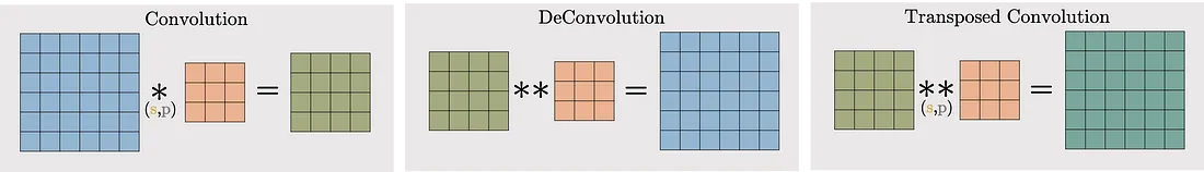
A transposed convolutional layer, is usually carried out for upsampling i.e. to generate an output feature map that has a spatial dimension greater than that of the input feature map. And I will tell you that if you understood the standard convolution, you already understood the transposed convolution. The transposed convolutional layer is also defined by the padding and stride.

Implementing a transposed convolutional layer can be better explained as a 4 step process:

1. Calculate new parameters z and p’
2. Between each row and columns of the input, insert z number of zeros. This increases the size of the input to (2i-1)x(2i-1)
3. Pad the modified input image with p’ number of zeros
4. Carry out standard convolution on the image generated from step 3 with a stride length of 1

In PyTorch, the torch.nn.ConvTranspose2d class represents a transposed convolutional layer. You can include it in your models as follows:

torch.nn.ConvTranspose2d(in_channels, out_channels, kernel_size, stride=1, padding=0, output_padding=0, groups=1, bias=True, dilation=1, padding_mode='zeros')

I will assume that if you are already here you should understand what each parameter means, they are the same as the Conv2d, there is only one new output_padding that handles ambiguities when the stride is greater than one, ensuring the output shape is as desired.

The animations below explain the working of convolutional layers for different values of stride and padding (find more here).

Pixel Shuffle

This layer is useful for upsampling without transposed convolutional layers, we can do the upsampling inside a network with normal convolution layers followed by a pixell shuffle layer. This is useful for super resolution tasks. This layer was proposed by Shi et al. (2016), for the task of super-resolution.

Again, I recommend you review Animated AI's animations and their explanation of the module. Likewise, I place the animation here to have it at hand.

What you have just seen is pixel shuffle, but the interesting thing about this module is that we can return, yes, unshuffle, this is how it looks (additionally I place the complete animation).

2x2 Pixel Unshuffle	2x2 Pixel Shuffle/Unshuffle Loop

This module has already been implemented by us and the code explanation is available here 🥳! You can also find the Pytorch implementation if you want to use it in one of your networks (also Unshuffle).

2.6 Autoencoder

The U-Net architecture (Ronneberger et al., 2015), originally proposed for biomedical image segmentation, stands out as one of the most significant contributions in the evolution of deep learning models. This design has proven effective for tasks requiring both detailed localization and global context understanding, such as image reconstruction and segmentation.

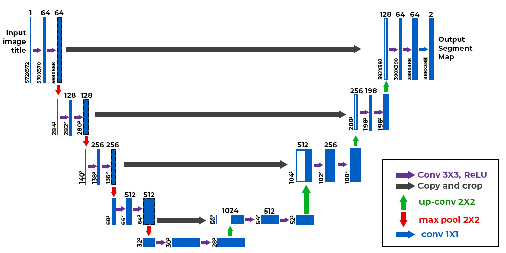
We also have this architecture implemented in our repository 🥳! I also provide you with the following two resources where they explain and code the architecture (Spanish, English, there are a lot more, of course).

U-Net is the autoencoder used as a reference by (dare I say) all research. An autoencoder learns two functions: an encoding function that transforms the input data, and a decoding function that recreates the input data from the encoded representation [20] to recover an output as similar as possible to the original input. This architecture is important because it serves to understand the intuition behind encoder-decoders (although encoder-decoders are not the same as autoencoders). All autoencoders are encoder-decoder networks, but not all encoder-decoder networks are autoencoders. The following image is taken from here.

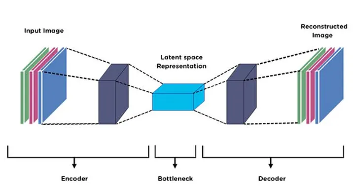
Encoder-decoder: This is a more general architecture used in tasks where the input is transformed to an output that may not be the same as the original. Here, the encoder takes the input and compresses it into a latent representation, while the decoder expands it to produce an output that may have a different shape. It is even used in applications such as generative models (e.g., context encoders) and machine translation (e.g., transformer).

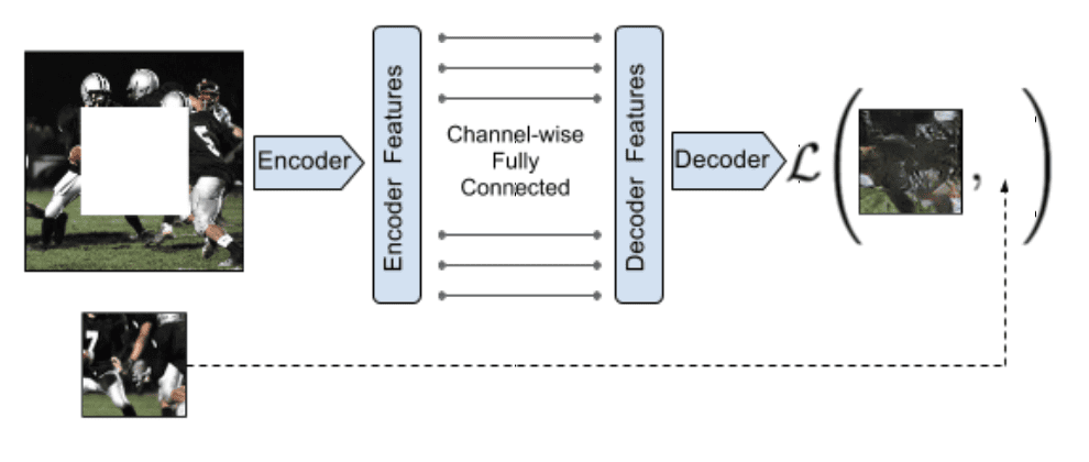Context Encoders	Transformer architecture

An excellent explanation of the Transformer architecture starts here.

---

This module was built by @guillepinto, if you have questions, complaints or constructive criticism contact me.